Thermodynamic Power Cycle Analysis
Jakcson Harvey (11/18/2022)INTRODUCTION
In thermodynamics, a heat engine is a device that can exchange heat energy and work. Thermodynamic Power Cycles (TPC) are the form of heat engine which convert heat energy to usable mechanical work (typically by rotating a turbine shaft). A Working Fluid, which can transmit heat and work by nature, facilitates the energy exchange. All heat engine systems operate using the same core principles. However this complicates things from an analysis standpoint since we now have 2 intercoupled degrees of freedom. The two mechanisms by which energy exchange \(dU\) can occur: \[dU_{therm} = Tds\] \[dU_{flow} = Pdv \] \[dU = Tds+Pdv\] Kinetic \(KE\) and potential \(PE\) also have effects but to less a degree. In reality this means for a slight amount of work Pdv (fluid) energy we can transport large amounts of Tds (entropy driven heat) between thermal reservoirs (between a heat source and heat sink)- however what a power cycle also does is siphon Pdv work off of that Tds as it innevitbaly deteriates into the void entropic relief. All heat engines operate as follows:
From ground state (A)- The fluid is compressed \(dU_{s=constant}\) (\(Pdv\) spent)
- Heat is transferred into the system from a high-temperature source
- A portion of the heat gets converted to work
- The remaining waste heat is rejected to a low-temperature sink (often the surrounding environment)
- The process is a cycle
In this report, we will consider the two types of closed power cycles:
- The Brayton cycle, in which the working fluid is in a gaseous state the entire cycle.
- The Rankine cycle, in which liquid and vapor phases of the working fluid are present at different points in the process
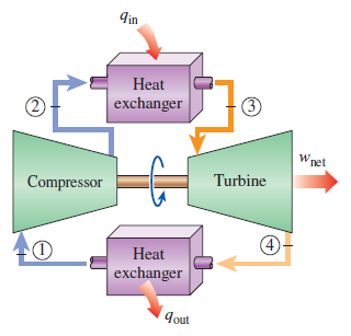
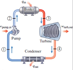
The most basic forms of these cycles are shown below in figure 1 and 2. In both cycles, the four processes involve (1-2) Work input to the system, (2-3) Heat into the system, (3-4) Work out of the system, (4-1) Heat out of the system. In an ideal cycle, the work processes are adiabatic, and the heat processes are isobaric.
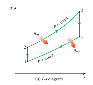
An essential tool in power cycle analysis is the TS diagram, in which temperature is plotted as a function of specific entropy (kJ/kg). The TS diagrams for the simple Brayton and Rankine cycles are below. The enclosed area of the processes corresponds to the net work of the cycle. Thus by increasing this area, we can increase the net work of the cycle.
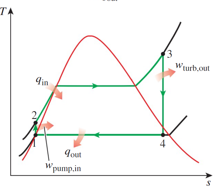
Noticing the “Dome” in the Rankine cycle diagram, which describes the phase of the working fluid. When fluid is in the dome, the fluid undergoes a phase change between liquid and vapor. The phase change is a constant pressure and temperature process (in the absence of external work). The change liquid-to-gas corresponds to a left-to-right process and vice versa. Along the left and right lines in the diagram, the fluid is a saturated liquid and saturated gas, respectively.
One way to conceptualize this is to think about a similar phase change process. Imagine a fully frozen glass of water is placed in a room temperature enironment and allowed to slowly warm. As the ice warms the temperature on the surface slowly rises to 0 C at which point these molecules begin to change phase. This consumes energy since you are decreasing the . Assuming this process occurs relatively slowly, the 2 phases of the water will be in equilibrium. Now consider: at any time before all the ice melts, will the temperature of the liquid water be greater than the temperature of the frozen water? The answer is no. Not until all of the ice melts can the temperature of the liquid rise above 0°C, the fluid's melting point. Often misunderstood, the melting and boiling temperature of a fluid (function of pressure) are points at which 2 phases of the fluid will coexist. Relevant to the Rankine cycle, when a substance is in the dome, the quality factor x reflects the mass ratio of the vapor and liquid phases present.
We also need to understand the regions above the dome. The dome's peak is the critical point above which the phase must be uniform, either a liquid or a solid. Above the dome and to the left of the critical point is the compressed liquid region, and to the right is the superheated vapor region.
Alternatively, there is no dome in the Brayton cycle since the working fluid is far above its critical point. Often, the working fluid in a Brayton cycle can be considered an ideal gas.
BACKGROUND
The fundamental equations associated with thermodynamics are known and well documented. The purpose of this paper is not to rederive these relationships; therefore, a certain level of familiarity is assumed for the reader. Nonetheless, this section presents several necessary concepts and equations used throughout the report.
If the reader is familiar with thermodynamic analysis, they should proceed to section Evaluation Section for the computational method presented.
First and Second Laws of Thermodynamics
All TPC systems must remain within limits set by the first and 2nd laws of thermodynamics. The 1st law is a familiar form of energy conservation, which states: energy is a thermodynamic property that must always be conserved.
The 2nd law is less intuitive and is often associated with the disorder of a system. From the author's perspective, disorder is a poor way of conceptualizing its implications in thermodynamics. Instead, the 2nd law implies that heat transfer has a preferred direction (hot to cold) and that preference has an intensity (quality). Furthermore, in the absence of external work, these statements are absolute. The second law consists of 2 equivalent statements:
- Heat will not transfer from a cold body to a hot sink without external work
- A cycle that receives heat from a high-temperature reservoir cannot produce net-work without rejecting some heat to a low-temperature sink (i.e., no system can convert 100% of the received heat to work)
Entropy, S, is a construct that enforces these rules. Furthermore, there is no entropy associated with adiabatic processes. In all systems, the entropy change of the internal system plus the entropy change of the surroundings must be greater than or equal to 0. A process with 0 entropy change is said to be isentropic, and is therefore reversible.
NOTATION
In most of this report, energy will be in Unit Mass Form, also known as "specific" form. The Total Energy, \(E\) [kJ], and specific energy, \(e\) [kJ/kg], are related by: \(e = E/m\), where m is the mass [kg]. It is typical to express energy in the time-rate form(\(d/dt\)) which is denoted by: \(\frac{d}{dt}E = \dot{E}\) [kW]. \(\dot{E}\) and \(e\) are related by \(\dot{E}=\dot{m}e\), where \(\dot{m}\) is the mass flow rate in [kg/s].
THERMODYNAMIC PROPERTIES
This section provides a brief review of thermodynamic properties and their implications. Intensive Properties are the mass-independent properties of a system \((T,P,\rho)\). These properties cannot be put into "specific" form as the relationship is meaningless. Extensive Properties are characteristic properties that depend on the system configuration. Meaning they are not innate to the fluid, rather a product of the conditions. Some examples of these properties are \(E\) and volume \(\mathbb{V}\). These properties can be put into "specific" form as they are a function of mass, and therefore of the form \(X = mx\), where \(X\) is the total properties and \(x\) is the specific property. It should also be noted that the specific volume \(\nu = \frac{\mathbb{V}}{m} = \frac{1}{\rho}\)
KEY RELATIONSHIPS
First, we review the definition of the Total Differential, $df$, of some function $f(x,y)$:
\[ df = \left(\frac{\partial f}{\partial x}\right)_ydx + \left(\frac{\partial f}{\partial y}\right)_xdy \]
We should also introduce the definition of enthalpy and the Gibbs relationships:
\[ h = u + Pdv \]
\[\begin{aligned} Tds &= du + Pdv\\ Tds &= dh - vdP \end{aligned}\]
We now take the time to further evaluate two special cases relevant to power cycles. When the working fluid can be considered an incompressible substance, the following relationships hold:
\[\begin{equation} \begin{aligned} \nu = \text{constant } \to dv &= 0\\ c_p(T) = c_v(T) = c(T) \to du &= c(T) dT \end{aligned} \label{incompRelations} \end{equation}\]
And from the definition of enthalpy in Eq \(\ref{enthalpy}\), we can say:
$$dh = c(T)dT + \nu dP$$
Alternatively, when the working fluid can be considered an Ideal Gas, intuitively, the first equation necessary to evaluate an ideal $$cp = c_v+R $$ $$k = \frac{c_p}{c_v}$$ $$du = c_vdT$$ $$dh = c_pdT$$ Finally, when an ideal gas with *constant specific heats* undergoes an **isentropic** process, we can say: $$\left(\frac{T_2}{T_1}\right)_{s=const} = \left(\frac{P_2}{P_1}\right)^{\frac{k-1}{k}}=\left(\frac{v_1}{v_2}\right)^{k-1}$$
CONTROL VOLUMES
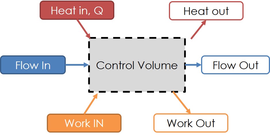
A general diagram for control volumes is provided in Fig 3, which can contain any given component in any TPC. We take the time now to express the energy balance and formulation for thermodynamic control volumes. We start by defining the energy transport by mass \(\theta\) and resultant flow energy \(E\):
\[ \begin{aligned} \theta = h + ke + pe = h + \frac{V^2}{2} + gz \end{aligned} \] \[ \begin{aligned} E_{mass} &= m\theta \textit{ (Amount)} \\ \dot{E}_{mass} &= \dot{m}\theta \textit{ (Rate)} \end{aligned} \]The basic principle of the First Law of Thermodynamics is \(E_{in} - E_{out} = E_{stored}\). We usually elect to evaluate the specific rate form of the equation \(\dot{e}_{in} = \dot{e}_{out} + \dot{e}_{stored}\). And at steady state, we know that \(\dot{e}_{stored} = 0\). To reduce the number of terms in the energy balance equation, we establish the convention:
\[ \begin{aligned} \dot{Q}_{net} &= \dot{Q}_{in} - \dot{Q}_{out} \\ \dot{W}_{net} &= \dot{W}_{out} - \dot{W}_{in} \end{aligned} \]Meaning that a positive net work or heat term correlates to energy exiting the system. The full energy balance for a control volume can then be expressed by:
\[ \begin{aligned} \dot{Q}_{in} + \dot{W}_{in} + \sum_{in}\dot{m}\theta &= \dot{Q}_{out} + \dot{W}_{out} + \sum_{out}\dot{m}\theta \\ \dot{Q}_{net} - \dot{W}_{net} &= \sum_{out}\dot{m}\theta-\sum_{in}\dot{m}\theta \end{aligned} \]