

TJLFEP.jl
A Julia port of TGLF-EP, the energetic-particle (EP) critical-gradient threshold model built on top of TJLF (the Julia port of TGLF). TJLFEP scans a scale factor on the EP pressure gradient until a marginally unstable Alfvénic mode appears, yielding the critical EP density/pressure gradients used for EP transport and stability studies.
It is a close, jointly-maintained translation of the Fortran GACODE add-on TGLF-EP (verified against it bit-for-bit), and adds a CUDA GPU eigensolver plus Julia-native autodiff (ad) solvers. On the reactor-relevant UCP_complete case these make TJLFEP substantially faster than a fully MPI-parallel Fortran CPU reference (-n 1280) — ~4–8× in node-hours at N_BASIS=32 — and, through the ad solvers, more accurate: they resolve the narrow-width (w<1) EP-driven Alfvén modes that Fortran misses at its default WIDTH_MIN=1 width floor. (Lowering WIDTH_MIN lets Fortran span those widths, but its linearly-spaced width grid and quantized factor grid still miss modes the Julia solvers land on via log-spaced width seeding and exact-AD root-finding.)
Which solver? Choose along two axes. Do you want to match Fortran or improve on it, and do you want the faithful value or a faster approximation?
| Faithful | Faster approximation | |
|---|---|---|
Match Fortran (w≥1 box) | :grid reproduces Fortran (~4.4×) | :ad :only approximates :grid (~8×) |
Extend Fortran (adds w<1 AE modes) | :ad :locate (default) (~1.7×) | :ad :wide (~5.4×) |
Multipliers are node-hours vs the fully MPI-parallel Fortran CPU reference (-n 1280, 10 CPU nodes) at N_BASIS=32 on the reactor-relevant UCP_complete case (the fair, node-count-normalized cost; see the benchmark below). The GPU advantage grows with eigenmatrix size (:grid reaches ~8× at N_BASIS=48), so it is largest for reactor cases at production N_BASIS; on the smaller DIII-D case the margins are thinner (see docs/README_DIII-D_example.md). :ad :locate is the production default (the ActorTJLFEP default) and reports the faithful narrow-width value.
For the full API reference, see the online documentation.
Capabilities
- Verification against Fortran TGLF-EP: run the same case through the canonical Fortran
TGLFEP_driverand Julia and overlay the results. - Run + validate on an
input.gacode+input.TGLFEPpair. - Database generation on GPU (NVIDIA MPS, 1 radius/worker).
- Timing vs
N_BASISbenchmark (Fortran CPU / Julia CPU / Julia GPU), for both thegridand autodiff (ad) solvers. - Sysimage build + run (removes JIT cost for production).
- FUSE-native IMAS
ddpath: run from an IMAS data dictionary using the same preprocessing/runTHDroutines as theinput.gacodepath.
Repository layout
| Path | Contents |
|---|---|
src/ | The TJLFEP package (module TJLFEP). |
build/ | Run / verify / benchmark / sysimage scripts (see build/README.md). |
examples/ | Canonical DIII-D and ITER cases (see examples/README.md). |
utils/ | Preprocessing-comparison utilities (see utils/README.md). |
test/ | Regression tests, incl. the nb6 Fortran-match fixture. |
docs/ | Verification/reproduction notes + benchmark assets. |
Installation
Requires Julia 1.11+ (1.11.7 and the default NERSC juliaup Julia 1.12+ are both fine). TJLFEP depends on registered TJLF >= 1.2.4 (FuseRegistry); no TJLF checkout is needed.
cd TJLFEP
julia --project=. -e 'using Pkg; Pkg.instantiate(); Pkg.precompile()'
The GPU path requires CUDA >= 12.6 (the eigensolver calls cusolverDnXgeev).
On HPC systems Julia and CUDA are typically provided as modules (e.g. module load julia cudatoolkit/12.9 on Perlmutter, or a pinned julia/1.11.7). If your shared filesystem has a small or slow home directory, point JULIA_DEPOT_PATH at a larger scratch location before instantiating.
Depot-path gotcha (don't clobber your home depot). When
JULIA_DEPOT_PATHis unset, Julia defaults to~/.julia(where most users already have their packages/artifacts). A bareexport JULIA_DEPOT_PATH=$PSCRATCH/.juliareplaces that default, so Julia then looks only in scratch and silently stops seeing everything in your home depot. Always prepend/append instead of overwriting, and include$HOME/.juliaexplicitly:# keep the home depot (Julia's default) AND add scratch: export JULIA_DEPOT_PATH="$HOME/.julia:$PSCRATCH/.julia${JULIA_DEPOT_PATH:+:$JULIA_DEPOT_PATH}"The first entry is where Julia writes (precompile cache, downloads); later entries are search-only. This same rule is what lets a prebuilt sysimage find its JLL artifacts — see "Sharing a sysimage with other users" in
build/README.md.
Quick start
using TJLFEP

# File-based path (loaded standalone, TJLFEP stays light, no IMAS/FUSE):
runTHD("input.TGLFEP", "input.MTGLF", "input.EXPRO"; use_gpu=true)

# Directly from an input.gacode + scan-control input.TGLFEP:
runTHD_from_gacode("examples/DIIID_202017C42_500ms_v3.1/input.gacode",
                   "examples/DIIID_202017C42_500ms_v3.1/input_scan20_nb6.TGLFEP";
                   use_gpu=true)

# FUSE-native IMAS data dictionary (same gradient routines as input.gacode):
runTHD(dd, rho, OptionsDict; use_gpu=true)   # see examples/ITER/ITERstructExample.jl
On Perlmutter, the batch wrappers in build/ drive these on Slurm; start with cd build && sbatch run/batch_smoke_test.sh (capability 2). See build/README.md for the full per-capability script index.
Verification against Fortran
The Julia port reproduces the Fortran TGLFEP_driver SFmin profile to its printed precision on the DIII-D 202017C42_500ms_v3.1 case. The verification scripts default to the shared Fortran build at /global/cfs/cdirs/m3739/gacode_add_d3d/TGLF-EP (override TGLFEP_DIR).
cd build
sbatch verify/batch_debug_nb6_fortran_scan20_10n.sh   # Fortran reference
sbatch verify/batch_debug_nb6_julia_scan20_10n.sh     # Julia
# then overlay:
FORTRAN_DIR=... JULIA_DIR=... FILE_DIR=... ./verify/compare_debug_nb6_scan20.sh
Agreement at the scan radii: SFmin max relative error ~0.03%; α(dn/dr) ~0.5%. A self-contained smoke-level regression (test/runtests_regression_nb6.jl) checks one radius against the archived Fortran golden output. Full steps: docs/REPRODUCE_FORTRAN_MATCH.md; physics-parity notes: docs/FORTRAN_JULIA_COMPARISON.md.
Benchmark: cost vs NBASIS (UCP, SCANN=20)
Timing/accuracy on the reactor-relevant UCP_complete case (4 thermal ion species + energetic particles), a 20-radius scan on Perlmutter with sysimages. This is the headline benchmark because the GPU eigensolver's payoff scales with the eigenmatrix size (species × N_BASIS): UCP's per-ky eigenmatrix is 2400² (complex) at N_BASIS=32 vs 1440² for DIII-D, so each eigensolve is several× heavier and the GPU pulls decisively ahead. The smaller DIII-D verification case, where the margin is thinner, is in docs/README_DIII-D_example.md.
Cost is reported in node-hours (nodes × wallclock), the fair, layout-independent metric (Fortran -n 1280 on 10 CPU nodes, the GPU tiers on 5 or 1). Each solver runs on its fastest parallel layout (rule of thumb: grid → MPS team, ad → in-process threads; an MPS team only adds overhead to ad).
The solvers, with node-hours vs the fully MPI-parallel Fortran (-n 1280) at N_BASIS=32:
| Solver | vs Fortran | What it computes |
|---|---|---|
:ad :only | ~8× | Approximates :grid: a smooth, de-quantized version of the w≥1 result (median :only/grid ≈ 0.9). Fast iteration only; misses the w<1 edge modes. |
:ad :wide | ~5.4× | Adds the narrow w<1 AE modes in one log-seeded pass; conservative (within ~1–2× of :ad :locate, never below it). Bulk NN-DB generation. |
:grid | ~4.4× | The verified Fortran-equivalent (kyhat × width × factor) sweep (thousands of eigensolves/radius). |
:ad :locate (default) | ~1.7× | Adds the narrow w<1 AE modes; the faithful narrow-width value. Production default. |
The ad solvers are grid-independent: rather than reading sfmin off the coarse factor grid, they locate the instability onset directly (Newton root-find with exact forward-mode AD derivatives). :grid/:ad :only stay in the Fortran w≥1 box; :ad :locate/:ad :wide additionally resolve the narrow-width (w<1) EP-driven modes it excludes (the entire sfmin reduction below grid, up to ~16× at the edge). Higher-fidelity internal reference tiers (robust_ad, and the nbasis-converged truth) sit above :ad :locate, which matches them essentially bit-for-bit; they are documented for reference in docs/AD_SOLVERS_AND_SEARCH_BOUNDS.md.
Accuracy: sfmin(IR) for all solvers at N_BASIS=32:
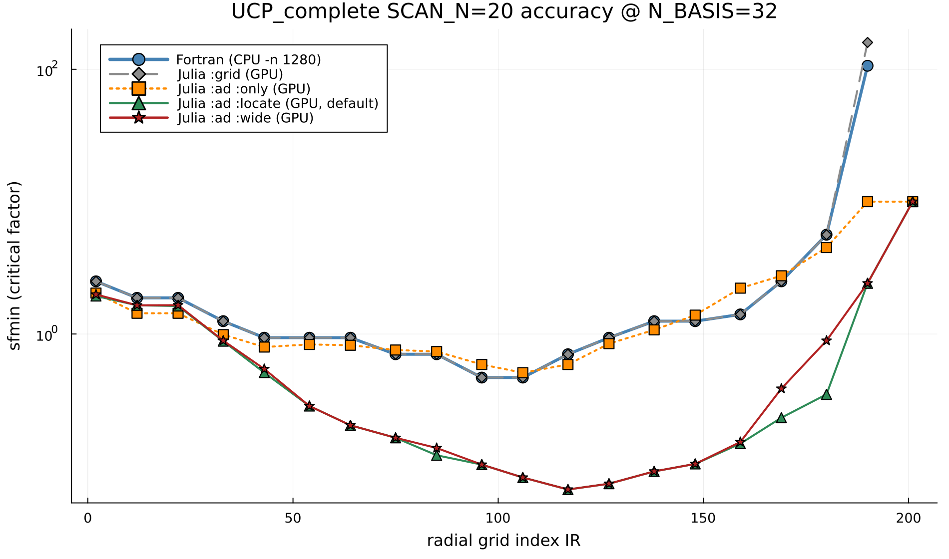
:grid (grey) reproduces the Fortran reference (blue) bit-for-bit, and :ad :only (orange) tracks it closely (the de-quantized w≥1 value). :ad :locate (green) and :ad :wide (dark red) drop well below grid into the narrow-width w<1 modes at the outer radii (IR ≳ 40; ~10× below grid at IR≈117, up to ~16× at IR≈180). :ad :wide stays within ~1–2× of :ad :locate and never below it. Colors and legend order match the node-hours plot below for quick cross-reference.
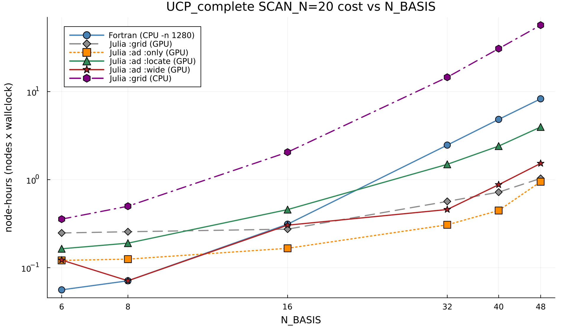
Absolute node-hours at N_BASIS=32, each solver on its fastest layout (Fortran -n 1280 on 10 CPU nodes; grid/:ad :only on 5 MPS GPU nodes; :ad :locate/:ad :wide on a 1-node backfill with 4 GPU workers draining a 20-radius queue): Fortran ≈2.47; :ad :only ≈0.31, :ad :wide ≈0.46, grid ≈0.57, :ad :locate ≈1.49 — so every GPU tier beats the fully-parallel Fortran (~8× / ~5.4× / ~4.4× / ~1.7×). Julia :grid on CPU (≈14.6, same 10 nodes as Fortran) is ~6× slower than Fortran: the GPU eigensolver is what makes the Julia port competitive. The GPU advantage grows with N_BASIS (Fortran is cheaper at N_BASIS ≤ 8, break-even is near 16, and the GPU pulls ~4–8× ahead by 32) as the eigenmatrix grows: at N_BASIS=48 (Fortran ≈8.29 node-hours) the margins are :grid ~8.0× (≈1.03), :ad :only ~8.7× (≈0.95), :ad :wide ~5.4× (≈1.53), :ad :locate ~2.1× (≈3.97). :ad :wide is ~3× cheaper than :locate at N_BASIS=32. The per-backend tables below give the raw wallclock seconds.
Fortran cannot run N_BASIS>32 without recompiling. Stock TGLF hard-caps the Hermite basis at a compile-time PARAMETER (nb=32); requesting more does not error — a put_switches sanity check silently resets the run to the default nbasis=4, returning garbage in seconds (the failure is only visible as an impossibly fast run). The N_BASIS=40/48 Fortran columns here required rebuilding the TGLF library with nb=48, nxm=95 (a full make clean rebuild — the gacode Makefile does not track Fortran module dependencies). TJLF/TJLFEP allocate the basis dynamically, so the Julia solvers run any N_BASIS unmodified.
Best-throughput layout depends on the solver (for these SCAN_N=20 runs):
:gridand:ad :only→ 5 GPU nodes. Per-radius cost is uniform, so spreading the 20 radii across 5 nodes (~4 radii/node) minimizes wallclock with no wasted node-hours.:ad :locateand:ad :wide→ 1 GPU node, backfill. Their edge radii take much longer (the narrow-widthw<1locate is triggered there), so a fixed multi-node split would leave nodes idle waiting on the straggler edge radii. Running a single node with 4 workers draining a shared 20-radius claim queue keeps every GPU busy and gives the lowest node-hours. AtN_BASIS=48the default 32-worker team OOMs the node's 256 GB host RAM, so the nb48:locate/:widerows run a halved team (MPS_TEAM=4, 16 workers) on 80 GB A100 nodes (-C gpu&hbm80g) — the fastest layout that fits.
Grid solver: Fortran CPU (10 nodes, -n 1280 = 128 ranks/node) vs Julia CPU (10 nodes, SlurmClusterManager) vs Julia GPU (5 A100 nodes, MPS team):
| N_BASIS | Fortran CPU (s) | Julia CPU (s) | Julia GPU MPS (s) | GPU speedup vs Fortran (wallclock) |
|---|---|---|---|---|
| 6 | 20.3 | 128.2 | 178.4 | 0.11× |
| 8 | 25.4 | 179.5 | 184.3 | 0.14× |
| 16 | 112.2 | 739.0 | 197.0 | 0.57× |
| 32 | 888.8 | 5243.7 | 407.5 | 2.18× |
| 40 | 1741.3 | 11082.4 | 518.9 | 3.36× |
| 48 | 2982.5 | 20489.1 | 743.9 | 4.01× |
(Wallclock here compares a 5-node GPU run to a 10-node -n 1280 Fortran run — half the nodes — so it understates the GPU, yet it still wins 2.18× at N_BASIS=32 and 4.01× at 48; the fair node-count-normalized margins are ~4.4× and ~8.0×. Julia :grid on CPU, on the same 10 nodes as Fortran, is a steady ~6–7× slower at every N_BASIS, so the GPU is doing the heavy lifting. The 40/48 Fortran times use the nb=48 rebuild described above; the 40/48 Julia CPU rows ran on a v2.0.13 CPU sysimage — the N_BASIS≤32 rows used an earlier bake — so there is a minor code-version seam in the CPU column only.)
:ad :only (bare w≥1 AD, no faithful confirm): Julia GPU (5 A100 nodes, in-process threads), vs the grid GPU path (both 5-node, so this wallclock ratio is apples-to-apples):
| N_BASIS | Grid GPU MPS (s) | :ad :only GPU threads (s) | :only vs grid-GPU (wallclock) |
|---|---|---|---|
| 6 | 178.4 | 87.4 | 2.0× |
| 8 | 184.3 | 90.3 | 2.0× |
| 16 | 197.0 | 119.8 | 1.6× |
| 32 | 407.5 | 220.9 | 1.8× |
| 40 | 518.9 | 320.8 | 1.6× |
| 48 | 743.9 | 681.7 | 1.1× |
:ad :only is ~1.6–2.0× faster than the grid MPS path in wallclock (narrowing to ~1.1× at N_BASIS=48, where the few-but-huge AD eigensolves stop amortizing their serial descent): it replaces the thousands of grid eigensolves/radius with a handful of AD Newton steps. Note this is the same ad solver run two ways: on an MPS team instead of threads it is slower, because the per-radius AD regions are small and the descent is sequential, so team-spawn/remote-call overhead never amortizes. Rule of thumb: grid → MPS, ad → threads.
Data: docs/plots/ucp_scan20_timing.csv. Reproduce with build/timing/submit_ucp_scan20.sh (Fortran -n 1280 + all GPU tiers). The smaller DIII-D verification case (bit-for-bit Fortran match) is in docs/README_DIII-D_example.md.
Spectrum diagnostic (PROCESS_IN=3)
Besides the critical-gradient threshold scans (PROCESS_IN=4/5), TJLFEP supports the TGLF-EP spectrum diagnostic (PROCESS_IN=3). It does not scan or search for a critical factor; it just computes the linear growth-rate / real-frequency spectra γ(ky), ω(ky) at fixed plasma conditions, by running the full TGLF transport model over a fixed ky grid (nky=30, ky=0.15, KY_MODEL=0, NBASIS=32) at three drives:
mode_in | file | drive |
|---|---|---|
| 1 | out.eigenvalue_m1 | background plasma + EPs (thermal gradients retained) |
| 2 | out.eigenvalue_m2 | EP drive only |
| 4 | out.eigenvalue_m4 | EP-only with TAE/EPM filtered (typically leaves ITG/TEM) |
Comparing the three shows which part of the spectrum is EP-driven (AE/EPM) vs thermal (ITG/TEM). With WIDTH_IN_FLAG=true the fixed WIDTH_IN is used; with WIDTH_IN_FLAG=false a TGLFEP_ky_widthscan (EP-only) first picks the max-growth-rate width (and marks kymark), then the spectrum is computed at that width.
Because it yields spectra rather than an SFmin/critical gradient, this mode is not routed through ActorTJLFEP (which would error); call TJLFEP directly. A single radius runs in a few minutes on a CPU login node; a full radial scan, a GPU run, or any long job should go to Slurm (NERSC login nodes are shared and kill heavy/long processes).
A ready example input is examples/DIIID_202017C42_500ms_v3.1/input_spectrum.TGLFEP (see also the manual test/smoke_spectrum.jl).
Quick login-node run (one radius, CPU)
module load julia/1.11.7
export JULIA_DEPOT_PATH="$HOME/.julia:$PSCRATCH/.julia${JULIA_DEPOT_PATH:+:$JULIA_DEPOT_PATH}"
cd TJLFEP
julia --project=. -t 8 --startup-file=no
using TJLFEP # loaded standalone, TJLFEP stays light (no IMAS/FUSE), CPU-only here
CASE = "examples/DIIID_202017C42_500ms_v3.1"
gacode = joinpath(CASE, "input.gacode")
tglfep = joinpath(CASE, "input_spectrum.TGLFEP") # PROCESS_IN=3
# run ONE radius (scan_index=1); writes out.eigenvalue_m{1,2,4} into out_dir
r = run_gacode_scan_task(gacode, tglfep, 1; out_dir="spectrum_out", printout=true)
r.spectra[1] # (ky, gamma, freq) for mode_in=1; [2]=EP-only, [4]=ITG/TEMgamma/freq are nky × nmodes matrices (row i = ky[i]). Useful threads scale up to ~nky=30 (the ky loop is threaded); keep it modest on a login node. For a few radii, loop scan_index over 1:SCAN_N.
Slurm (full scan, or GPU)
Use a job when running many radii, on GPU, or unattended:
#!/bin/bash -l
#SBATCH -N 1 -n 1 -c 128 -C cpu -q debug -t 00:30:00 -A m3739 -J spectrum
module load julia/1.11.7
export JULIA_DEPOT_PATH="$HOME/.julia:$PSCRATCH/.julia${JULIA_DEPOT_PATH:+:$JULIA_DEPOT_PATH}"
cd TJLFEP
julia --project=. -t 32 --startup-file=no -e '
  using TJLFEP
  CASE="examples/DIIID_202017C42_500ms_v3.1"
  for i in 1:SCAN_N    # set to your input’s SCAN_N
      run_gacode_scan_task(joinpath(CASE,"input.gacode"), joinpath(CASE,"input_spectrum.TGLFEP"), i;
                           out_dir="spectrum_out", printout=true)
  end'
For GPU, use -C gpu, load cudatoolkit, and pass use_gpu=true. At NBASIS=32 the per-ky eigenmatrix is (NS−NS0+1)·15·NBASIS = 1440² (complex), so the GPU eigensolver helps each solve, but the ky solves serialize on one GPU (no cross-ky batching), so the real GPU payoff is across many radii via the same inner=:threads/:mps_team multi-GPU layout used by the PROCESS_IN=5 scans.
Validation
test/runtests_regression_spectrum.jl compares the Julia spectra to a Fortran golden (test/fixtures/spectrum/out.eigenvalue_m{1,2,4}_r040); agreement is ~3e-5 relative. See test/fixtures/spectrum/README.md for how the golden was generated. Note the public Fortran TGLFEP_driver has a bug on the PROCESS_IN=3 + EXPRO path (q_scale uninitialized → zeroed q → DSYEV failure), so a one-line-patched reference binary was used.
Citation
If this software contributes to an academic publication, please cite it as follows:
T.F. Neiser, D. Sun, B. Agnew, T. Slendebroek, O. Meneghini, B.C. Lyons, A. Ghiozzi, J. McClenaghan, G. Staebler and J. Candy, TJLF: The quasi-linear model of gyrokinetic transport TGLF translated to Julia, APS Meeting Abstracts (2024)