Polyharmonic Splines (PHS)

Overview

Polyharmonic splines (PHS) are radial basis function (RBF) interpolants optimized for smooth approximation of multidimensional gridded data. They are particularly effective for smooth-on-log-scale data and when combined with custom reference functions, enabling physics-informed interpolation in specialized domains like quantum chemistry.

Key features:

• N-dimensional on uniform rectilinear grids (equal spacing per axis)
• C² continuous — local stencils blended across neighbouring nodes
• Analytical derivatives through the standard deriv keyword
• Stencil-based evaluation — cost independent of grid size
• Log-density transform — accurate near singularities (e.g., nuclear cusps)
• Custom reference functions — any callable ρ₀ with derivatives, or ConstantRef

See Differences from the other methods and current limitations for what PHS does not support yet.

Mathematical Foundation

This section summarizes the polyharmonic spline method. For full details, see the paper.

Basic PHS Interpolant

A polyharmonic spline is constructed as:

\[\omega(x) = \sum_i w_i \phi(\|x - x_i\|) + p(x)\]

where:

• \[\{x_i\}\]

  are $N$ stencil nodes (grid points)

• \[\phi(r) = r^K\]

  is the radial kernel ($K$ odd, typically $K=3$ for $\phi(r)=r^3$)

• \[p(x) = v_0 + v_x x + v_y y + v_z z\]

  is a linear polynomial augmentation

• \[w_i\]

  and $v$ are interpolation coefficients determined by solving:

\[\begin{pmatrix} \Phi & C^T \\ C & 0 \end{pmatrix} \begin{pmatrix} w \\ v \end{pmatrix} = \begin{pmatrix} \rho \\ 0 \end{pmatrix}\]

where $\Phi_{ij} = \phi(\|x_i - x_j\|)$, $C_i = (1, x_i)$, and $\rho = (\rho_1, \ldots, \rho_N)$ are data values.

Log-Density Smoothing Transform

For data with singularities or rapid variation (e.g., electron density near nuclei), interpolate the transformed function:

\[f(x) = \ln\left(\frac{\rho(x)}{\rho_0(x)}\right)\]

where $\rho_0(x)$ is a smooth reference function (e.g., promolecular density, empirical model, or physical constraint).

The interpolant is built on $f(x)$, which is smooth by design. Evaluation recovers the original density and derivatives via the chain rule:

\[\tilde{\rho} = \rho_0 \exp(f)\]

\[\tilde{\rho}_\xi = \rho_0 \left( f_\xi + \frac{\rho_{0\xi}}{\rho_0} \right)\]

\[\tilde{\rho}_{\xi\zeta} = \rho_0 \left( f_{\xi\zeta} + \frac{\rho_\xi \rho_\zeta}{\rho_0^2} + \frac{\rho_{0\xi\zeta}}{\rho_0} - \frac{\rho_{0\xi}\rho_{0\zeta}}{\rho_0^2} \right)\]

Blending for C² Continuity

Since stencils change discontinuously at grid node boundaries, a blend function combines multiple local interpolants:

\[\rho(x) = \frac{\sum_i w_i(x) \tilde{\rho}_i(x)}{\sum_i w_i(x)}\]

with smooth weight $w_i(x)$ that transitions from 1 at node $x_i$ to 0 at distance $a$ (blend range). This ensures $C^2$ continuity across the domain.

API Usage

Basic PHS Interpolation

using FastInterpolations

# Define grid and data
x = range(0.0, 1.0, 20)
y = range(0.0, 1.0, 20)
data = [sin(xi) * cos(yj) for xi in x, yj in y]

# Create interpolant
itp = phs_interp((x, y), data; stencil_size = 8, degree = 3)

# Query
val = itp((0.5, 0.3))
grad = itp((0.5, 0.3); deriv = (DerivOp(1), DerivOp(0)))

With Custom Reference Function

# Define reference density
ref = ConstantRef(1.0)  # simple constant reference

# Build PHS with log-transform
itp = phs_interp((x, y), data; 
    reference_interp = ref, 
    stencil_size = 8, 
    degree = 3)

# Stored data is log(ρ/ρ₀); evaluation returns ρ
val = itp((0.5, 0.3))  # ≈ ρ(0.5, 0.3), not log(ρ)

Custom Reference with Analytical Derivatives

Create a callable reference function supporting the interface ref(q) and ref(q; deriv=(DerivOp(...), ...)):

struct MyReference
    # ... state ...
end

(ref::MyReference)(q; deriv=nothing) = begin
    if deriv === nothing
        # return value
        return ρ₀(q)
    else
        # return derivatives based on deriv tuple
        # deriv = (DerivOp(n₁), DerivOp(n₂), DerivOp(n₃))
        # means ∂^(n₁+n₂+n₃)ρ₀/∂x^n₁ ∂y^n₂ ∂z^n₃
        ...
    end
end

itp = phs_interp((x, y, z), rho_data;
    reference_interp = MyReference(),
    stencil_size = 8,
    degree = 3)

Parameters and Tuning

Measured accuracy/speed trade-offs for these parameters are collected in PHS Performance and Tuning.

Example: Quantum Chemistry

The script scripts/phs/phs_density_comparison.jl demonstrates PHS for electron density interpolation in a phenol dimer, recreating Figure 2 in the paper. It uses:

• Data: DFT-computed electron density (B3LYP/TZ2P, 0.236 Bohr spacing). The committed grid is a 30×42×30 sub-box of the full 75×113×70 grid around the O7…H21 path at the original spacing, with a 12-node margin on every side; the comparison only evaluates along that path, so the error statistics and the figure are identical to the full-grid run
• Reference: Analytical promolecular density (sum of PBE atomic densities from critic2)
• Validation: Comparison of density, gradient, and Laplacian along a hydrogen-bond path

The resulting plot shows exceptional agreement with analytical values, even near nuclear cusps and steep features:

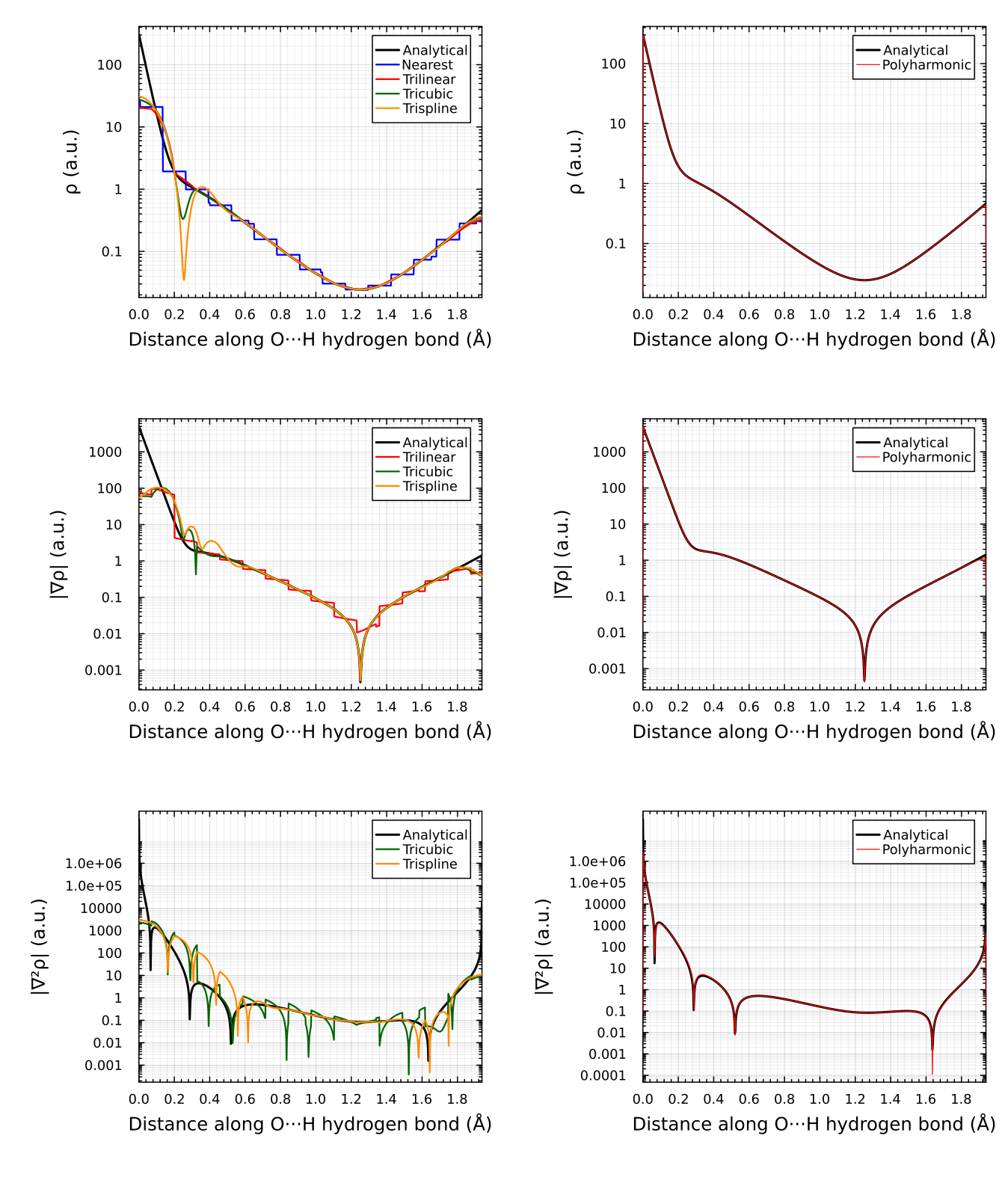
Left column: Standard 3D interpolation methods (nearest, linear, cubic spline, cardinal) vs. analytical DFT values. All exhibit spurious oscillations and errors near the nuclei. Right column: PHS with log-density transform and promolecular reference. Smooth, accurate across the domain, with only minor deviations very close to nuclei.

Polyharmonic spline interpolation was added specifically for applications to physical systems with singularities and steep features, where they achieve better relative results. The results show that PHS with log-density transform and a promolecular reference achieves orders of magnitude better accuracy than nearest, linear, cubic spline, and cardinal interpolation for both the density and its derivatives, even near nuclear cusps, at the expense of higher computational cost.

Running the Example

The script automatically downloads wavefunction files on first run:

julia --project=scripts scripts/phs/phs_density_comparison.jl

To get timings that don't include JIT compilation and stencil caching, run the script twice:

julia --project=scripts -e 'include("scripts/phs/phs_density_comparison.jl"); include("scripts/phs/phs_density_comparison.jl")'

This generates phs_density_comparison.png and demonstrates:

• Loading XYZ atomic geometry
• Building PromolecularRef from critic2 PBE wavefunctions
• Constructing PHS interpolant with log-transform
• Evaluating density, gradient, Laplacian analytically
• Batch evaluation for performance

The accuracy and timing tables for this example are in PHS Performance and Tuning.

Differences from the other methods and current limitations

PHS is a local radial-basis method rather than a piecewise polynomial, so parts of the common API do not apply or are not implemented yet:

• Uniform grids only. The stencil geometry is built from one spacing per axis, so results are only correct when every axis is equally spaced. Non-uniform axes are accepted without error but the interpolant then no longer reproduces its own data (tracked as a @test_broken pin).
• No boundary conditions. Continuity comes from stencil blending, not from end conditions; there is no bc keyword.
• Search and hints. Uniform grids locate the base node in O(1); non-uniform grids use a binary search. search is only used for out-of-domain checks and hint is ignored.
• Derivatives use the standard deriv keyword. The gradient/hessian/laplacian helpers do not support PHS yet.
• Not implemented: adjoint operators, integrate, complex-valued data, the 1-D bare-vector constructor, GriddedQuery/GridIdx queries, and ClampExtrap/WrapExtrap (use NoExtrap or FillExtrap).
• Known issue: first derivatives evaluated exactly on a grid node are inaccurate. This and the items above are tracked as @test_broken pins in test/test_phs_broken_pins.jl.

References

• Paper: Otero-de-la-Roza, A. Finding critical points and reconstruction of electron densities on grids. J. Chem. Phys. 156, 224116 (2022).
• critic2: Database of PBE all-electron atomic densities