Multi-Dimensional Interpolation

FastInterpolations.jl supports 2D, 3D, and N-dimensional interpolation on rectilinear grids. The API generalizes the 1D case: where 1D takes x, ND takes (x, y, ...) as a Tuple.

Prerequisite

This section assumes familiarity with the 1D API. Every 1D concept (methods, BCs, extrapolation, derivatives) extends to ND via Tuples.

Quick Start

using FastInterpolations

# Define a 2D rectilinear grid and data
x = range(0.0, 2π, 20)
y = [0.0, 0.3, 0.7, 1.0, 1.5, 2.0]   # non-uniform
data = [sin(xi) * cos(yi) for xi in x, yi in y]

# Interpolant API (recommended)
itp = cubic_interp((x, y), data)
itp((1.0, 0.5))                         # scalar query

# One-shot API
cubic_interp((x, y), data, (1.0, 0.5))  # same result

The Tuple Rule

Every 1D argument becomes a Tuple in ND. This applies uniformly:

Concept	1D	ND
Grid	`x`	`(x, y)` or `(x, y, z)`
Query (scalar)	`xq`	`(xq, yq)`
Query (batch)	`xqs::Vector`	`(xqs, yqs)`
BC	`bc=CubicFit()`	`bc=(CubicFit(), PeriodicBC())`
Extrap	`extrap=ClampExtrap()`	`extrap=(ClampExtrap(), WrapExtrap())`
Derivative	`deriv=DerivOp(1)`	`deriv=DerivOp(1, 0)` for ∂f/∂x
Search	`search=AutoSearch()` (default)	`search=AutoSearch()` (default) or per-axis tuple (e.g., `search=(AutoSearch(), AutoSearch())`)

Broadcast rule: A scalar value is broadcast to all axes. bc=CubicFit() is equivalent to bc=(CubicFit(), CubicFit()) in 2D.

Available Methods

All four interpolation methods support ND:

Method	Function	BC Required?	Continuity
Constant	`constant_interp((x,y), data)`	No (`side` only)	C⁻¹
Linear	`linear_interp((x,y), data)`	No	C⁰
Quadratic	`quadratic_interp((x,y), data)`	Yes (1 per axis)	C¹
Cubic	`cubic_interp((x,y), data)`	Yes (2 per axis)	C²

Grid Types

Each axis can independently be a Range (uniform, O(1) lookup) or Vector (non-uniform, O(log n) lookup). This allows heterogeneous grids:

x = range(0.0, 1.0, 100)          # uniform → O(1)
y = [0.0, 0.1, 0.4, 0.9, 1.5]    # non-uniform → O(log n)
itp = cubic_interp((x, y), data)   # mixed grid works

Data Orientation

data must satisfy size(data, d) == length(grids[d]) for each dimension.

Query Modes

Scalar Query

itp((0.5, 1.0))  # returns a single value

Batch Query (SoA — Structure of Arrays)

xqs = range(0.0, 1.0, 50)
yqs = range(0.0, 2.0, 50)
itp((xqs, yqs))  # returns Vector of length 50

Batch Query (AoS — Array of Structures)

points = [(0.1, 0.2), (0.3, 0.4), (0.5, 0.6)]
itp(points)  # returns Vector of length 3

Any Indexable Container (Query Protocol)

ND batch evaluation accepts any container type whose elements are indexable points. Types with standard length, getindex, and eltype semantics work zero-config:

using StaticArrays

# Vector{SVector} — works out of the box
pts = [SVector(0.1, 0.2), SVector(0.3, 0.4)]
itp(pts)  # returns Vector of length 2

# AbstractVector query also works for scalar calls
itp(SVector(0.5, 1.0))  # single-point evaluation

For custom containers where Base semantics differ (e.g., SoA-style wrappers), override three functions:

import FastInterpolations: _query_length, _query_extract, _query_eltype

_query_length(q::MyQueries)      = ...   # number of query points
_query_extract(q::MyQueries, k)  = ...   # k-th point (any indexable)
_query_eltype(q::MyQueries)      = ...   # scalar floating type (e.g. Float64)

Value types vs Query types

This is orthogonal to Custom Value Types (Duck Typing), which governs what types can be interpolated (Tv). The query protocol governs what container types can hold query points.

Visualization (2D)

2D interpolants have built-in plot recipes:

using Plots
itp = cubic_interp((x, y), data)
plot(itp)  # heatmap with grid nodes and gridlines

Example — Method Comparison

Comparing constant, linear, quadratic, and cubic interpolation on a non-uniform 2D grid:

using FastInterpolations, Plots

f(x, y) = sin(2π * x) * cos(2π * y)

xs = [0.0, 0.1, 0.4, 0.5, 0.82, 1.0]
ys = [0.0, 0.1, 0.2, 0.5, 0.8, 0.9, 1.0]
data = [f(xi, yj) for xi in xs, yj in ys]

itp_const = constant_interp((xs, ys), data)
itp_linear   = linear_interp((xs, ys), data)
itp_quad  = quadratic_interp((xs, ys), data; bc=MinCurvFit())
itp_cubic = cubic_interp((xs, ys), data)

kw = (c=:RdBu, clims=(-1,1), ratio=:equal, xlims=(0,1), ylims=(0,1))

itps = (itp_const, itp_linear, itp_quad, itp_cubic)
plot((plot(itp; kw...) for itp in itps)..., layout=(2,2), size=(950, 900))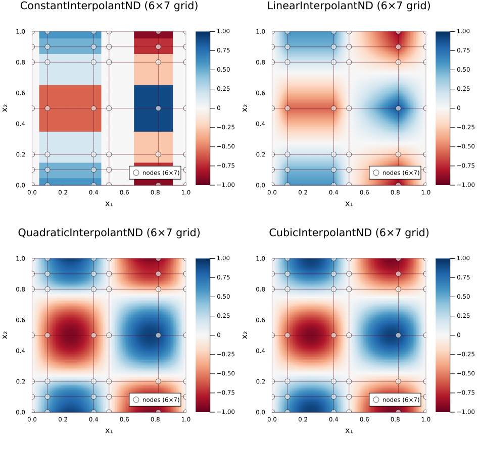

Custom options: show_nodes, show_gridlines, resolution, node_color, gridline_style. Use help_plot(itp) to discover all options.

Unified API: `interp` / `interp!`

The interp function provides a single entry point for N-dimensional interpolation with per-axis method specification. It supports both homogeneous (all axes same method) and heterogeneous (mixed methods per axis) interpolation.

# Homogeneous: auto-dispatches to CubicInterpolantND (same as cubic_interp)
itp = interp((x, y), data; method=CubicInterp())

# Heterogeneous: cubic on axis 1, linear on axis 2
itp = interp((x, y), data; method=(CubicInterp(), LinearInterp()))
itp((0.5, 0.3))  # evaluate
gradient(itp, (0.5, 0.3))  # analytical gradient works

One-Shot (Zero-Allocation)

Evaluate without creating an interpolant — ideal for hot loops with changing data:

# Scalar one-shot
val = interp((x, y), data, (0.5, 0.3); method=(CubicInterp(), LinearInterp()))

# Batch one-shot
vals = interp((x, y), data, (xqs, yqs); method=CubicInterp())

# In-place batch
interp!(output, (x, y), data, (xqs, yqs); method=CubicInterp())

Per-Axis Options

Each axis can have its own method, boundary condition, and extrapolation:

itp = interp((x, y, z), data3d;
    method = (CubicInterp(bc=PeriodicBC()), LinearInterp(), QuadraticInterp()),
    extrap = (WrapExtrap(), ClampExtrap(), NoExtrap()),
)

For full details, see the dedicated Unified API Guide.